More about metrics: turf in 2 dimensions

I’ve written about the attractions of metric units and how facility with those units can make turfgrass management easier. I want to explain this a bit more, especially as it is related to fertilizer and to water, first discussing 2 dimensional surfaces.

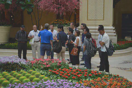
At a seminar in Macao (presentation slides and handouts here), this very subject came up. I was discussing turfgrass fertilizer, which is vastly simplified because turf surfaces can be considered as a 2 dimensional area, square meters (m²) or square feet (ft²) or whatever.

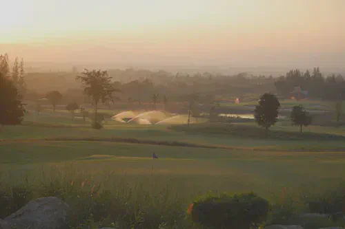
But with landscapes, as we saw at the interior gardens (above) and outdoor gardens and golf course (below) at the Venetian Macao, it is very much an irregular and inconsistent 3 dimensional space.

These landscapes are impressive, but they resist simplification. When applying fertilizer, for example, should we apply it on a per plant basis? Or on a size of plant basis? Or on a gound area basis? Plus there are so many different species, each, presumably, with some different nutrient requirements.

With turfgrass surfaces, we don’t really have to consider those complications. Compared to landscape plants, turfgrass surfaces are simple. No matter where we are in the world, and no matter what grass type is being grown, we can express a number of important metrics in 2 dimensional terms.

I like to use one square meter (1 m²) as the base unit in 2 dimensional space. That is, I take a turf surface, such as the zoysia putting green pictured below, and consider it in terms of length (1 dimension) and width (1 dimension). Combining the length and width, we have 2 dimensions, and can consider the flat surface with those dimensions.

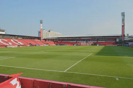
This goes for any turfgrass surface. Golf course putting greens, lawns, football fields – we often ignore the rootzone, and ignore the volume of the aboveground plant parts, and simply consider the flat 2 dimensional area.

We then express inputs to the turfgrass surface in terms of mass or volume as applied to a 2 dimensional space. For example, the annual nitrogen amount supplied to a turfgrass area might be 10 g N m^-2, which is equivalent to 2 lbs N 1000 ft^-2. We would be thinking of how much mass of something is applied per area. Turf is irrelevant here, because we could apply a mass of something to a certain area of parking lot, or of lawn, or of bare soil. It is just mass per area.

That’s easy, and we use those units all the time. Irrigation can be thought of in the same way. I often think of water in these terms. The consumptive water use of the grass is the evapotranspiration. In general one needs to supply something similar to the consumptive water use in order to keep grass actively growing. Water use (evapotranspiration) is expressed as a depth (1 dimension), just as precipitation is expressed as a depth (mm). We now have 3 dimensions, because we have a depth applied to an area, but with the metric system this is pretty easy to convert back to a mass or volume per area. No calculator required.

Let’s say we have ET of 4 mm, and we want to supply that as irrigation. 4 mm equals 4 L spread across 1 m², so for a 500 m² area, we would need 2000 L of water.

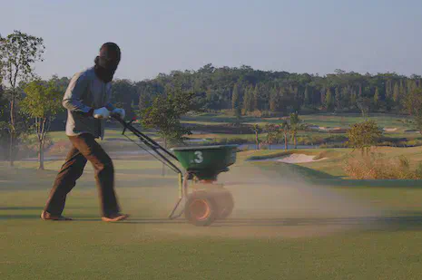
For topdressing sand, we could do the same type of expression. Topdressing sand may be applied at 100 g m^-2. For a 500 m² area, that would require 50 kg of sand.

Fertilizer, water, sand—applied as a mass or volume to a 2 dimensional area—this isn’t anything new.

But there is more to it than this, for the turf in reality is growing in a 3 dimensional space. Being able to convert the amount applied at the surface into units that express changes in the 3 dimensional space of the rootzone is quite useful. Being able to relate changes in the rootzone to simple units of how things are usually applied at the surface is also quite useful. Coming up, I’ll write about turf in 3 dimensions, and explain how I go about making some of these conversions on the fly, and why I find the metric system so useful in this regard.