Total organic matter testing on putting greens: sample number and sample volume
Cale Bigelow asked me an important question last month. I’d suggested that measuring the total organic matter over time is a way “to simultaneously produce a putting surface with the desired characteristics while minimizing the amount of disruptive work done to the putting surface.”

Cale asked about the sampling, specifically the number of cores to take and the sample volume.
The quick answer is here.
I recommend taking a minimum of five subsamples per green
I recommend testing a minimum of three greens
I recommend using a core sampler with a minimum diameter of 2 cm and a maximum diameter of 4 cm. I prefer 3 or 4 cm samplers; most golf courses have samplers closer to 2 cm in diameter.
Each subsample is approximately 6 cm3 with a 2 cm sampler to a 2 cm depth, 14 cm3 with a 3 cm sampler, and 25 cm3 with a 4 cm sampler. The total sample size, then, comes to about 30, 70, or 125 cm3, respectively, when gathering five subsamples with 2, 3, or 4 cm diameter samplers.
Jim Murphy suggested to me that combined small subsamples should, at a minimum, sample a total area of 4 square inches (25 cm2). This suggests a minimum volume for these samples should be 50 cm3. The reason for this minimum is to capture the effect of aeration holes based on the typical spacing for those holes.
Here’s the long answer, with some explanation of why I recommend that amount of sampling, and what type of precision to expect when a certain number of subsamples are collected.
I’m using terminolgy here of subsample and sample. By subsample I mean the many cores I might take from a green, placing them all in the same bag to be measured at the lab in a single test. Each of the cores I’ll call a subsample. The subsamples all combined together I call the sample. And if I sometimes call a subsample a sample, I hope you’ll be able to infer my meaning from the context.
Kauffman et al. have an interesting article about this called “Field sampling warm-season putting greens for thatch-mat depth and organic matter content.” They measured organic matter to a depth of 1 inch (25 mm) using large (10 cm diameter) core samples, and they got standard deviations ranging from 1.9 to 5.2 g kg-1 (that’s 0.19% to 0.52% OM). When I’ve measured individual samples from greens, I’ve found standard deviations from 3 to 21 g kg-1 (that’s 0.3 to 2.1% OM).
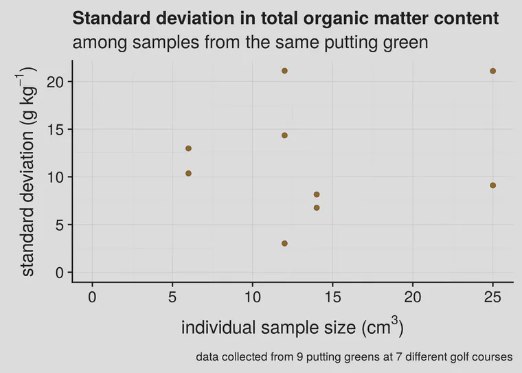
I’ve done this with small coring tools or soil profilers, and the standard deviation tends to be higher than reported by Kauffman. However, they worked with cup cutter samples having a volume of 196 cm3. In addition to that, I’d like to point out two things from Figure 1. First, at these relatively low sample sizes, which one gets from 2, 3, or 4 cm diameter soil samplers, there doesn’t appear to be a relationship between standard deviation and sample size. Second, there is variation that is inherent to the putting greens (or to the different golf courses) themselves.
This variation between courses is an important consideration. Because we expect every course to have a different amount of variation, it will be useful to look at the average number of samples required, for what we might expect on an average course. That’s the approach I took in this analysis, and is also why I’ve taken such a long time to come up with an answer that I was satisfied with to respond to Cale’s straightforward question.
I wanted to answer this question: based on the data I’ve collected so far, given the observed variability in the samples that were collected, how many subsamples do I need to get a mean that’s within plus or minus 5 g kg-1 of the mean of that area, given a possible subsample number of n = 1, 2, 3 … up to N?
I’m using mass values for OM here, to be consistent; in the units that OM is usually reported, 1% organic matter by weight would be 10 g kg-1. So if I measured a total OM in the top 2 cm—I think this can be denoted as OMT2 to indicate it it total OM (the T) and at a 2 cm depth (the 2)—and found it was 7.3%, that’s the same as an OMT2 of 73 g kg-1.
I’d like to sample to be confident that the OM measurement I make will be within 5 g kg-1 above or below the OM that I’ve measured previously. And importantly here, I’m expecting that the OM changes over time, so what I really want to do is be sure that I am getting an OM measuring that is no more than 5 g kg-1 away from the OM. We can’t really measure the real number—to do that we’d have to dig up the entire green and test all of it. So we do sampling, and calculate some statistics to find out some probabilities related to the samples that we do have.
I took the data from the individual subsamples that I’d collected from the nine different greens, and ran a multilevel model in Stan to find the highest probability values for the mean and standard deviation for each green, given the data that were observed. Then I simulated soil sampling from those greens with 1 subsample per green. This calculation found the expected OMT2 value I would get if only one subsample of small size were taken. Then I simulated what the mean OMT2 would be if two subsamples were taken. Then for three. And four. All the way up to 40 subsamples.
There is variation in the OMT2 on each of those greens. So if I take only one subsample, there is a lot of variation in what the mean value could be. If I take two subsamples, more of the variability in the green is within my sample, so the mean value gets a little more accurate. It keeps getting more and more accurate until I’ve dug up the entire green with samples, but I don’t want to do that. I need to stop sampling at some point.
At each number of subsamples—at 1, 2, 3 per green, all the way up to 40—I instructed the computer to calculate an 89% highest posterior density interval (HPDI). That interval contains 89% of the probability mass for the posterior distribution of the parameter values in the model, given the data that I collected.
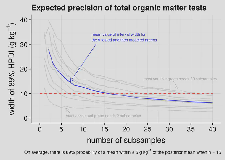
I’ve plotted this in Figure 2 as lines that go from from left to right, for each of the nine greens that was tested for individual subsamples, and included the mean line (in blue) which is what I expect for the average green.
What Figure 2 shows, in plain terms, is a width of the error margin on the vertical y-axis and how this changes as more samples are collected. For the average green, when I take 5 subsamples, the 89% interval is about 18 g kg-1. That’s plus or minus about 9 g kg-1. With 10 subsamples the interval is about 12 g kg-1. And at 15 subsamples the interval gets to what I’d like to see, which is plus or minus 5 g kg-1—an interval width of 10 g kg-1.
For any one green, it seems that collecting five subsamples will get an 89% interval for the mean within 10 g kg-1 plus or minus. If there are five subsamples, and the OMT2 is 8.3%, then I’m 89% confident that the mean of that area is within the 7.3% to 9.3% range. After one has measured three greens, each with five subsamples, now the 89% interval is about 10 g kg-1, so if I measured 8.3%, I now expect it to be within the 7.8% to 8.8% range.